
It’s finally time we shed some light on the technicalities behind this powerful tool. It took me some time digesting all these materials and I have to thank all the people who helped me understanding these passages. We will identify the differentials of the AHSS for spin-bordism (since it’s the one I need for my thesis), but the method we are going to use can be generalised to any AHSS, provided we have enough informations about the cohomology group of the spectra involved.
Since we will make an extensive use of this tool, it’s important that we clarify some technicalities about it. Our first aim is to prove the following lemma, which can be found as Lemma 2.3.2. page 27 in [Tei92]
Lemma 1
Let 

- The differential
is the dual of
- The differential
is reduction mod
composed with the dual of
.

We start with a definition:
Definition 1. An homology operation is a natural transformation between homology functors.
We call them stable if they commute with the suspension isomorphism, in analogy with the well-known stable cohomology operations. Now we want to relate this operations with the more famous cohomology operations, and we will do it as follows:
Lemma 2. Let 


Proof. By Yoneda lemma, we know that stable cohomology operations 


Since we used a map of spectra, the natural transformation preserves the suspension isomorphism (See [Rud] page 69) and it represents a stable homology operation by definition. Now let 


Therefore we created a cohomology operation, and after checking carefully the construction of such duality, it’s clear that these two assignations are one inverse of the other.
Now we want to give a construction of the AHSS in such a way that the differentials are clearly induced by maps of spectra. This is done in the paper [Mau] of Maunder, where the author build a version of the AHSS via an exact couple given by the Postnikov tower of the (co)homology theory. It’s clear that the construction done there (for spaces) can be lifted to the setting of spectra. He then identifies the differentials with 
Recall this result.
Theorem. Serre’s Theorem on the cohomology of 

- Let
be the mod


We are ready now to prove Lemma 1
Proof. Using the inclusion of the bottom cell 


In fact we are interested in differentials which start at most at the second row, since the third is trivial thanks to 
-
. In this case, the homology operation is classified by elements of
, where
is the Eilenberg-MacLane spectrum which represents singular homology with coefficients
. By definition,
. In fact the Steenrod algebra is well understood, and we know that the cohomology group we are interested in is generated by the Steenrod square
, where
denotes the sphere spectrum. We can consider the following commutative diagram given by the Spanier-Whitehead Duality:
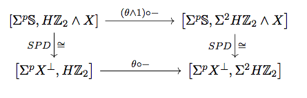 Where
Where is the map representing the stable homology operation
given by
where
is the duality
and
the multiplication given by the ring spectrum structure. This is (under the duality isomorphism) the well-known Kronecker pairing which in the case of field coefficient is a perfect pairing. For this reason we can identify
with the dual of
, and
. After plugging in some test-space (as done in [Tei92]), one realises that it’s not the trivial operation, therefore the claim.
. Here the reasoning is a little bit more involved. First of all, one has to realise that now we are interested in elements of
, which by definition is
. Therefore we need to compute this last cohomology group. Using the isomorphism
we need to figure out how does the
look like for big enough
. By Serre’s Theorem , we have that
, where
is the fundamental class. It’s easy to see that the colimit is given by the equivalence class of this element, therefore we have only two possible homotopy classes of map of spectra, the trivial one, and the one induced by
. As above, by a careful choice of test space, one can see that
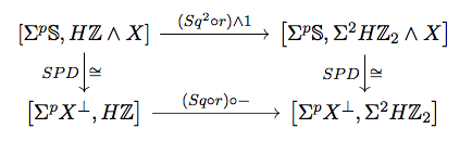 Now notice that
 . By definition, an element
can be represented by a map
. The effect of composition with
it’s the well-known reduction modulo
is given by the dual of the Steenrod square
We can give a nice description of the horizontal edge homomorphism in the AHSS for Oriented and Spin Bordism. Actually this can be generalised to other bordism theories, but we are interested in these two.
Definition 2. Let 


![[M,f] \mapsto f_*[M]](https://s0.wp.com/latex.php?latex=%5BM%2Cf%5D+%5Cmapsto+f_%2A%5BM%5D&bg=ffffff&fg=777777&s=0&c=20201002)
This map is clearly natural.
We start by recalling the geometric interpretation of the
Lemma 3. Let 


![[M,\partial M, f] \mapsto [\partial M, f_{|\partial M}]](https://s0.wp.com/latex.php?latex=%5BM%2C%5Cpartial+M%2C+f%5D+%5Cmapsto+%5B%5Cpartial+M%2C+f_%7B%7C%5Cpartial+M%7D%5D&bg=ffffff&fg=777777&s=0&c=20201002)
Proof. See the observation in [Rud] page 289.
The Steenrod-Thom map can be easily generalized to a map 

![[M, \partial M,f] \mapsto f_*[M,\partial M]](https://s0.wp.com/latex.php?latex=%5BM%2C+%5Cpartial+M%2Cf%5D+%5Cmapsto+f_%2A%5BM%2C%5Cpartial+M%5D&bg=ffffff&fg=777777&s=0&c=20201002)
Notice that the following diagram commutes
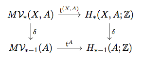
Since ![\delta f_*[M,\partial M] = f_*\delta [M,\partial M]=f_*[\partial M]](https://s0.wp.com/latex.php?latex=%5Cdelta+f_%2A%5BM%2C%5Cpartial+M%5D+%3D%C2%A0f_%2A%5Cdelta+%5BM%2C%5Cpartial+M%5D%3Df_%2A%5B%5Cpartial+M%5D&bg=ffffff&fg=777777&s=0&c=20201002)


We are now ready to prove the second main result (Prop 7.23 page 292 in [Rud])
Proposition. The edge homomorphism:

is given by the Steenrod-Thom homomorphism.
Proof. First of all, notice that the edge homomorphism is a stable homology operation. In fact if we use the exact couple given in [Mau] to define the AHSS, every map involved is clearly a stable homology operation. Therefore it has to be represented by an element in ![[M\mathcal{V},HZ]\cong Z\langle u\rangle](https://s0.wp.com/latex.php?latex=%5BM%5Cmathcal%7BV%7D%2CHZ%5D%5Ccong+Z%5Clangle+u%5Crangle&bg=ffffff&fg=777777&s=0&c=20201002)


![\left[\Sigma^p S , M\mathcal{V} \wedge X\right] \xrightarrow{n \cdot u\wedge 1} \left[\Sigma^p S , HZ \wedge X\right]](https://s0.wp.com/latex.php?latex=%5Cleft%5B%5CSigma%5Ep+S+%2C+M%5Cmathcal%7BV%7D+%5Cwedge+X%5Cright%5D+%5Cxrightarrow%7Bn+%5Ccdot+u%5Cwedge+1%7D+%5Cleft%5B%5CSigma%5Ep+S+%2C+HZ+%5Cwedge+X%5Cright%5D&bg=ffffff&fg=777777&s=0&c=20201002)
Since clearly 


Bibliography:
[Tei92], P. Teichner, Topological four-Manifolds with Finite Fundamental Group, PhD thesis
[Rud], Rudyak, On Thom spectra, Orientability, and Cobordism, Corrected 
[Mau], C.R.F. Maunder, The spectral sequence of an extraordinary cohomology theory, Mathematical Proceedings of the Cambridge Philosophical Society 59, 1963
[Ser], J.-P. Serre, Cohomologie modulo 2 des complexes d’Eilenberg-Maclane, Comment. Math. Helv. 27 (1953), 198-232.
